Reverse-Engineering The Discounted Cash Flow (DCF) Valuation

Learn how to value stocks by reverse-engineering the discounted cash flow method. Includes a free downloadable Excel sheet.

Nov 29, 2024

Dear reader,

Welcome to this new edition of Investing Topics.

In today’s edition, we’ll dive deeper into stock valuation, building on my previous post, How to Value Stocks using Discounted Cash Flow (DCF). This time, we’ll focus on the reverse DCF method.

While the DCF method can offer valuable insights, most experienced investors would agree it has its flaws.

It’s sensitive to assumptions—garbage in, garbage out. The discount rate can be tricky and difficult to comprehend. Additionally, calculating a terminal value after a forecast period of 5-10 years implicitly assumes no excess returns beyond that point, which can lead to the undervaluation of high-quality stocks.

The reverse DCF solves the problem of estimating the discount rate, and I’ll also be expanding on the standard DCF.

What you’ll Read Today

Recapping the DCF
Why Reverse-Engineer?
Reverse DCF in Practice
Conclusion

Recapping the DCF

Valuation, at its heart, is about determining the present value of all future cash flows. Valuing a stock boils down to forecasting those cash flows and then discounting them to their value today. Why, again, do we discount cash flows?

The reasoning is simple:

Cash today can be spent or invested to generate more capital, making it more valuable now.
Inflation decreases the purchasing power of future cash. A dollar today buys more than a dollar in the future.
Future cash flows are uncertain and carry risk—there’s no guarantee you’ll receive them.

By forecasting and discounting cash flows, we estimate a company’s intrinsic value.

However, there are things to take into consideration. Forecasts are inherently biased, and no valuation will be accurate. Estimation errors—or just being flat-out wrong—are likely possibilities.

So why value a stock at all when you’re guaranteed to be wrong?

Because every investor is wrong. It’s about being less wrong than others.

Since my initial post about DCF valuation, I’ve adopted two additional tools to help tackle its shortcomings.

Sensitivity Analysis
- One big flaw in a single DCF is the assumption of one scenario playing out. A sensitivity analysis allows you to explore a range of possibilities. For instance, instead of assuming revenue will grow by 10% the coming five years, you can model growth between 5-15%. This helps reduce estimation errors and helps you prepare for both conservative and optimistic scenarios. We’ll also include different scenarios for the operating margin, as that is another important determinant of cash flow.
Dynamic Forecast Period
- I’ve come to realize that a forecast period of 10 years can be limiting. It implies the company stops generating above-average growth after year 10. However, many high-quality companies manage to grow revenue faster than the typical 2-3% terminal growth rate well beyond the forecast period. This explains why these companies often appear overvalued in a DCF: much of their value lies beyond those initial 10 years.
  As an investor, it is your task to estimate how long a company can sustain growth above the terminal rate. Importantly, don’t try to predict the most likely scenario, but predict the scenario you’re most comfortable with—in other words, be conservative in your forecast period assumption.
  Further, analyze factors like: industry growth potential, competitive advantages, reinvestment levels through R&D and capital expenditures, and guidance and analyst forecasts.
  A company with high reinvestment in an immature and growing market, for example, should have a relatively longer forecast period.

By modeling multiple scenarios with varying growth and operating margin assumptions, and extending the forecast period thoughtfully, your DCF becomes more robust.

But there is still one last problem in a traditional DCF: the discount rate.

Why Reverse-Engineer?

Reverse-engineering a DCF involves using the current stock price to solve for the discount rate. This rate then represents the implied annual expected return, letting you judge whether the stock is attractive. If the expected return exceeds your hurdle rate—say, the S&P 500’s expected return—you buy the stock.

Let me explain.

In a traditional DCF, the formula below is used to calculate the intrinsic value of a firm.

The discount rate, represented by r, is derived using the WACC formula. From there, you plug in the cash flows and terminal value, and voilà, you get an intrinsic value. You can then compare this value to the market price to determine if the stock is over- or undervalued.

The reverse DCF takes a different approach. While the formula stays the same, instead of calculating the firm’s value, you solve for the discount rate. In this case, the stock price, or market capitalization, becomes the value. By solving for r, you arrive at the expected return from the current stock price, which is the annual return you can anticipate over the forecast period. Depending on your goals, you would then buy the stock only when the expected return exceeds your specific rate.

This method eliminates the need to calculate the discount rate using the WACC formula, which can be flawed due to the unrealistic assumptions of the CAPM model.

Using sensitivity analysis, you’ll get a range of potential outcomes for r, the annual expected return. Ideally, even the most conservative scenario should have a high expected return to justify the investment, but that’s rare.

In this approach, the stock price becomes a valuable tool for estimating the expected return. Ironically, the stock price itself tells you whether it’s over- or undervalued.

Reverse DCF in Practice

I often find myself understanding a topic better when learning with an example. That’s why we’ll dive into one now, using Salesforce, the CRM leader, as our guinea pig.

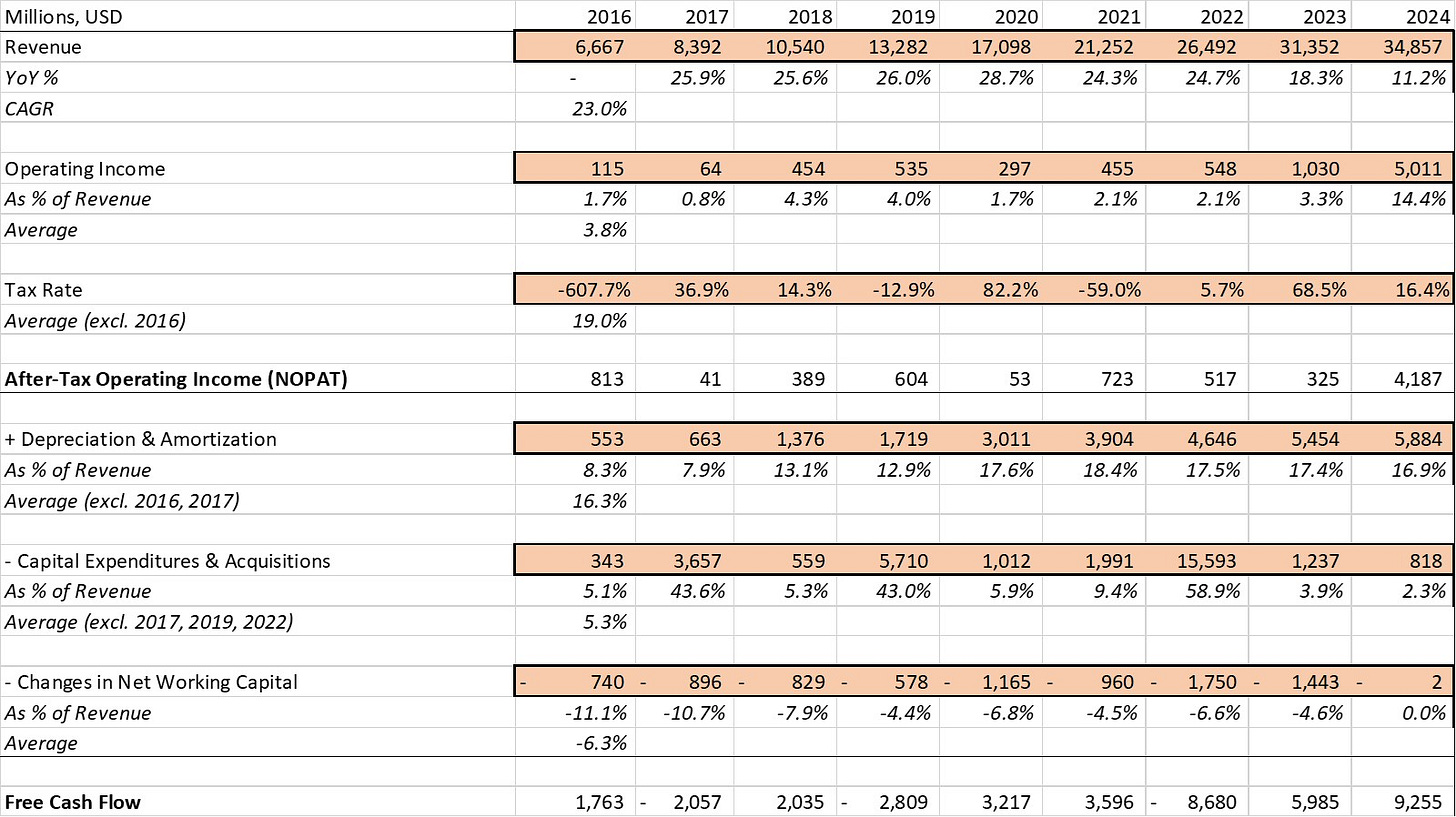
Just like a standard DCF, the first step involves collecting key data. I won’t go into detail here—if you’re unsure what to gather or how to calculate free cash flow, head back to my earlier post on the traditional DCF.

Having computed historic free cash flow, you must choose a forecast period. I’ve chosen a 20-year forecast for Salesforce, reflecting its mature growth phase and the expectation that its revenue growth will outpace the terminal rate during this period.

Next, we’ll make varying revenue and operating margin assumptions. Revenue typically slows over time, which is why we’ll make assumptions for different time periods. In our base case, Salesforce’s revenue grows by 9% annually in the first five years, after which it slows down to 7%, 5%, and 3%.

For operating margins, we assume gradual expansion from 19.7% (management’s guidance) in fiscal 2025 to 30% by year 20 in our base case.

Using these assumptions, we calculate After-Tax Operating Income (NOPAT) with a tax rate of 19%, Salesforce’s average in recent years. Free cash flow is derived by adding depreciation and amortization (D&A) and subtracting capital expenditures, acquisitions, and changes in net working capital (NWC).

A few remarks about the forecast:

D&A as a % of revenue is assumed to remain flat, which might be overly generous.
The forecast assumes no major acquisition, which may be unrealistic given Salesforce’s acquisitive track record.
It projects changes in NWC will gradually trend to 0%, consistent with historical patterns.

We now have free cash flow forecasts and a terminal value. This is all similar to a standard DCF, but here’s where we’ll take a turn.

Instead of calculating the discount rate using the WACC formula, we’ll compute the implied share price by summing the present value of forecasted free cash flows and terminal value, subtracting debt and adding cash, and dividing that by the number of shares outstanding.

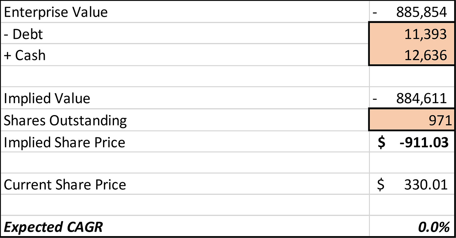
Initially, this will yield a nonsensical number (a negative share price) because the discount rate is still 0%.

Enterprise Value and Implied Share Price are negative because the Terminal Value is negative using a discount rate of 0%.

As seen in the image above, we now have the implied share price with a discount rate (Expected CAGR) of 0% and we have the current share price of Salesforce below.

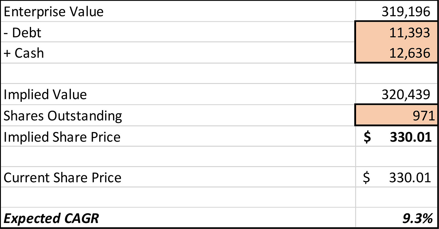
Using the Excel Solver tool, we can adjust the discount rate such that the implied share price matches Salesforce’s current share price.

The outcome is a 9.3% discount rate.

How should you interpret this number?

If you were to buy Salesforce at today’s price, and the base case assumptions hold true, you can expect an annual return of 9.3%.

I hope you can see the value in this—if you’re comfortable with the assumptions you’re making, and the implied discount rate meets your return targets, you can pull the trigger and buy.

Now, we can also play around with our sensitivity analysis. For instance, I believe an operating margin of 36% by year 20 is possible. With those assumptions, the discount rate increases to 9.7%.

Faster revenue growth in an optimistic scenario further pushes the rate to 10.4%.

Importantly, however, be careful not to tweak assumptions to match your desired outcome—it’s a common trap to avoid.

If you’ve set a hurdle rate, the reverse DCF can even help identify target prices at which you would buy. For example, let’s say you’re comfortable with Salesforce’s base assumptions and aim for an annual return of at least 10%, you would adjust the price until the discount rate reaches 10% or higher. In this case, the target price would be approximately $290, below the current price of $330.

Conclusion

The reverse DCF takes the traditional DCF a step further. In my opinion, this approach provides more valuable insights into a stock’s valuation, making it a valuable tool to add to your arsenal. Use it with caution, and make sure you’re comfortable with the assumptions you’re making.

Below is a downloadable Excel sheet which includes the Salesforce example we’ve gone through. It’s entirely free.

Reverse DCF Salesforce

26.8KB ∙ XLSX file

Download

Thank you for reading, and I hope this post gave you valuable insights into stock valuation. Let me know if you were already familiar with the reverse DCF or not!

Summit Stocks

Discussion about this post