Monte Carlo Valuation, the Damodaran Way

Modeling asymmetry, uncertainty, and risk, using Monte Carlo simulation

Today we continue with Monte Carlo simulation, the solution to single-point fair value DCF models. Monte Carlo helps investors measure asymmetry, quantify risk, and make better portfolio decisions.

Using a practical model inspired by the work of Aswath Damodaran, also known as the “Dean of Valuation,” we will walk through the Monte Carlo model step-by-step.

Let’s begin.

---

Quick Refresher: What Monte Carlo Does

The biggest flaw in most valuation models today is their single-point fair value outcome. You fill in your assumptions, hit enter, and out comes one number.

But that number is almost certainly wrong.

The future isn’t a fixed outcome. It’s a range of possibilities. Valuation, at its core, is about discounting all future cash flows, but there are countless ways those future cash flows could unfold.

Some scenarios look great, others not so much. A good model should reflect that uncertainty.

Monte Carlo simulation fixes this. It doesn’t give you one answer, but a distribution of outcomes, each tied to different assumptions about the future. Thousands of scenarios, each with its own fair value.

This used to be impractical due to a lack of computing power. Today it isn’t. Yet most investors still cling to the past.

Build a Base Case Valuation Model

Before you can simulate thousands of scenarios, you need a single working model.

Yes, that’s somewhat ironic, but you need a baseline and an actual DCF model in place.

I’ve recreated Damodaran’s Apple model as a reference, but with updated numbers. I’ve also added invested capital explicitly, as well as a dynamic sales-to-capital ratio.

Click to expand

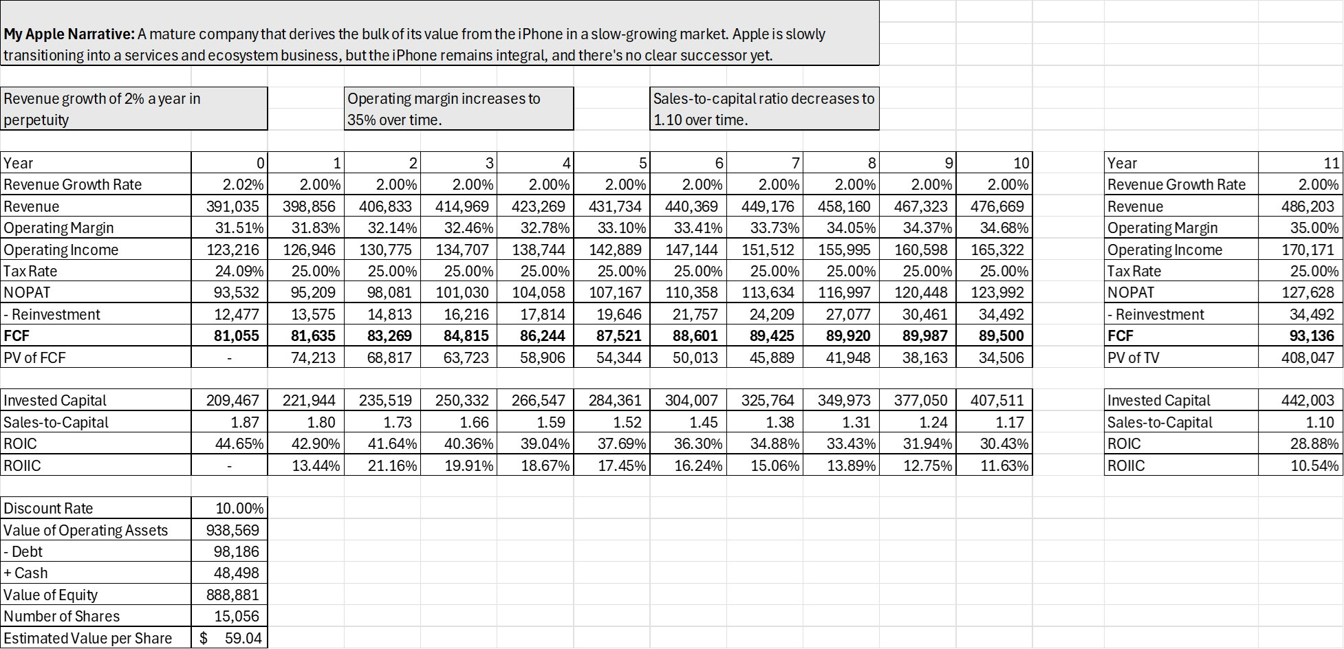
Key assumptions are:

1. Revenue grows at 2% annually into perpetuity

2. Operating margin expands to 35% as services outpace hardware

3. Sales-to-capital declines over time, reflecting mean reversion and a fading moat.

This isn’t anything new yet, but it gives us something to work with.

Identify Key Value Drivers

Before collecting data, we need to ask: which variables actually matter?

In my model, I fix the discount rate at 10%, as that’s my hurdle. Damodaran uses a variable rate, but it doesn’t have a significant impact on valuation.

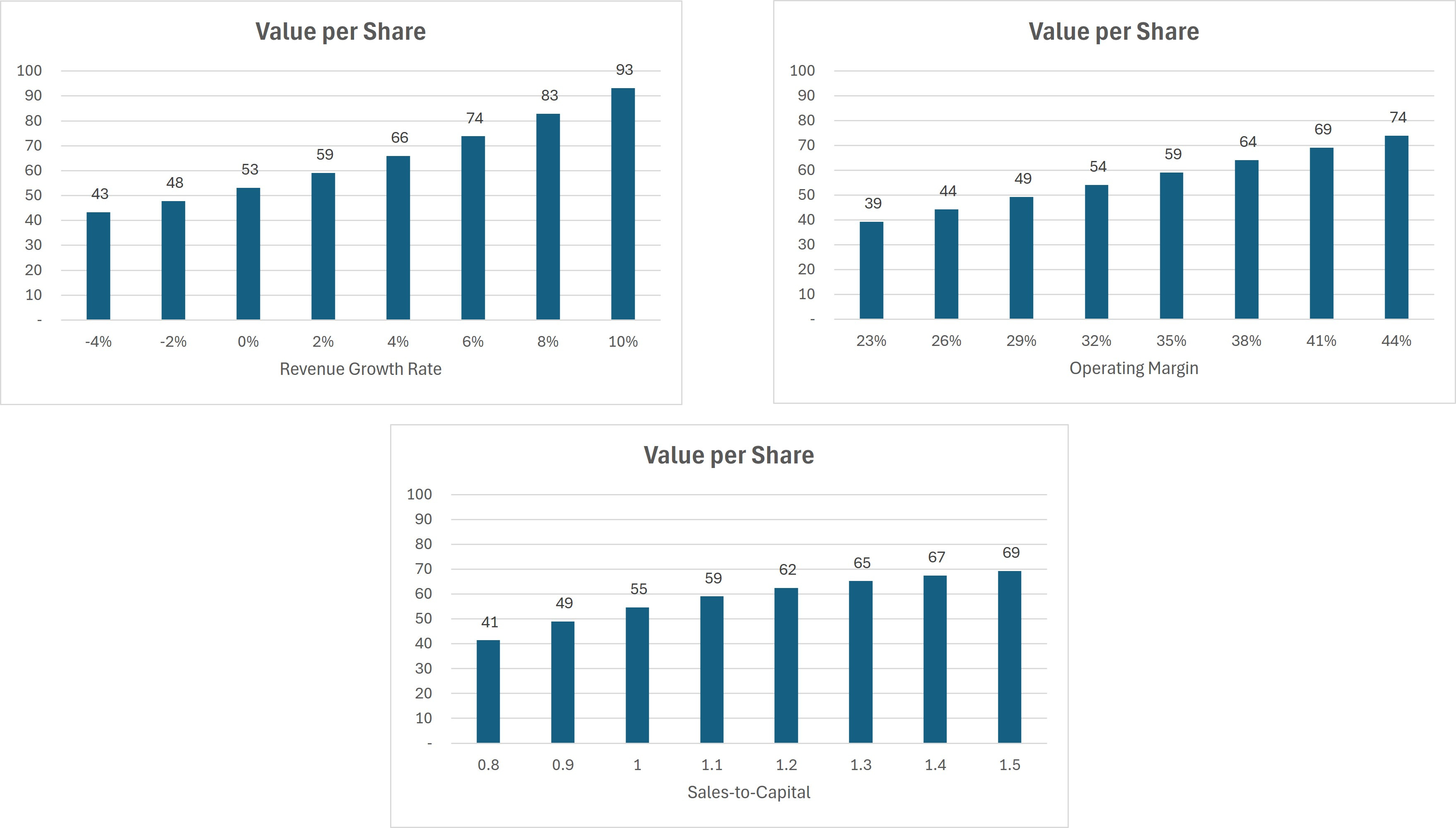
Sensitivity testing shows that revenue growth has the biggest effect on Apple’s valuation, but operating margin and sales-to-capital matter too. In Damodaran’s version, sales-to-capital is stable and thus has little impact. In my model, I assume it declines, so it plays a much larger role.

In short, all three variables are important and should be modeled as distributions.

Click to expand | Sensitivity testing for the three variables reveals that all three have a large impact on value per share

Collect the Data

Following Damodaran’s framework, we collect data in three ways:

1. Historical

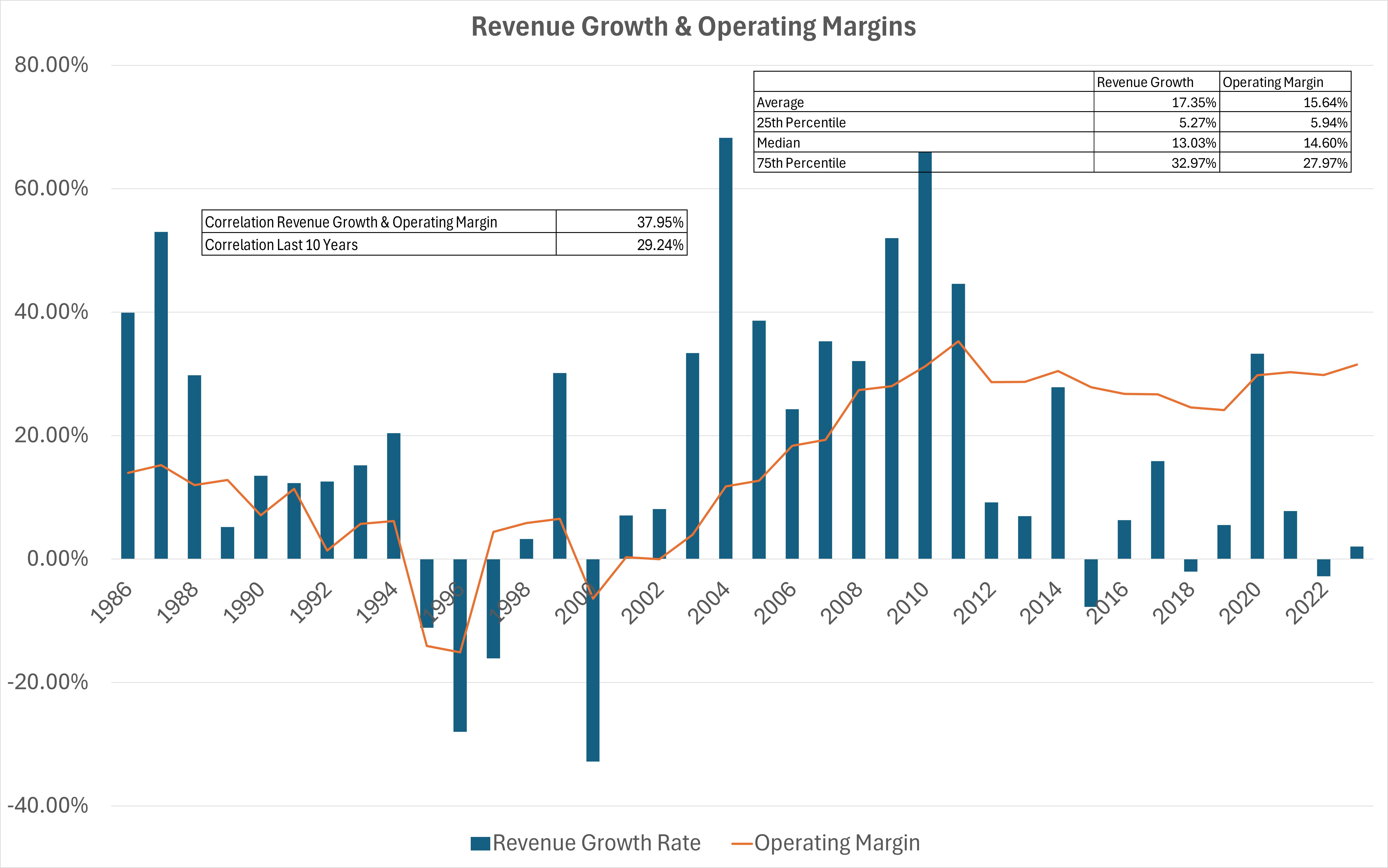
By analyzing Apple’s own track record of revenue growth and operating margin, we find some important insights. From 1986 to 2024, Apple’s average revenue growth rate was 17%, driven by the early growth phase. Over the past ~15 years, growth is clearly slowing, which is natural at Apple’s scale. During that same period, the operating margin has remained roughly flat.

Moreover, we see a visible correlation between revenue growth and margin, which will be useful later. Specifically, the correlation over the full period is 38%, and over the last 10 years, 29%.

2. Cross-Sectional

Damodaran suggests looking at peers in similar lifecycles. For this, I borrow Damodaran’s work, which analyzes the growth rate of tech firms older than 25 years, similar to Apple. He finds a mean and median growth rate of ~5%, while the 75th percentile is just below 10%. Importantly, 26% of firms had negative growth rates.

Source

3. Intuition

The data has give us a useful range, but intuition and common sense will help us narrow it down. A company at Apple’s size isn’t growing at 15%+ anymore. Even 10% growth is extremely generous.

So: -2% to 10% is our range for revenue growth.

Choose Distributions

With our value drivers defined, the next step is assigning a distribution to each variable, reflecting the range of possible outcomes and their likelihood.

There are several common distribution types worth knowing, such as binomial, uniform, triangular, normal, and lognormal. Each has different uses depending on how you think the future will play out.

1. Revenue Growth Rate

We’re assuming a range from -2% to 10%. We could treat each outcome as equally likely (uniform distribution), but that doesn’t seem realistic. If we think 2% is the most likely growth rate, most outcomes should cluster around that. A 10% growth rate is possible, but it should be rare.

A distribution shaped like a lognormal distribution is a better fit. It captures the skewness, where small positive growth is common, but large upside is increasingly unlikely.

2. Operating Margin

Margins have historically hovered around 30%, and I expect them to remain in that range. A triangular distribution works well here:

• Minimum of 25%

• Mode (the value that occurs most often) of 30%

• Maximum of 35%

Importantly, this means that operating margin in the final year will be between 25-35%, but most often close to 30%

3. Sales-to-Capital

This metric reflects how much capital Apple needs to reinvest to sustain growth. Again, I’m using a triangular distribution:

• Minimum of 1.1

• Mode of 1.3

• Maximum of 1.5

A higher ratio implies Apple maintains a stronger moat over time. A lower one suggests competitive pressures or structural decline in returns.

Run the Simulation

With distributions in place, we can already run some simulations.

Using 10,000 scenarios, we generate the following distribution of estimated fair values per share:

Click to expand | Generated using Crystal Ball (free trial). A great tool but expensive, which is why we’re building this directly into Summit’s Analytics.

The results are clear. Under most scenarios, Apple seems overvalued. The minimum value is $39.54, the maximum $603.11, but the 90th percentile is just $68.31. In other words, the scenario with the maximum value is extremely unlikely to happen. Most outcomes cluster somewhere between $50-60.

But we’re still missing one piece of the puzzle: correlation. In the above simulation, we’ve assumed that revenue growth and margins are independent. But as revenue grows, margins often expand too, thanks to operating leverage. In Apple’s case, we’ve already seen there’s some degree of correlation in the historical data.

After introducing a positive correlation of 0.3 between revenue growth and margins, the distribution tightens, but the result doesn’t drastically change. The new minimum is $39.82, the maximum $339.80, and the median and mean remain within the $50-60 range.

Click to expand

Interpretation and Takeaways

A single-point fair value gives you a two-way view: the stock is either over- or undervalued. That’s simplistic and often misleading.

Monte Carlo shows the full picture. In Apple’s case, it’s not just overvalued; we now understand how overvalued and we know the range of Apple’s valuation.

Now imagine Apple were trading at $50, which is right around the 25th percentile of our simulations. That tells us a few things: in 75% of outcomes, the stock would be overvalued. Downside is limited at 20% (because the minimum value is ~$40). And the potential upside is a lot higher than this 20% downside (with the maximum at ~$340).

That’s what’s called an asymmetrical setup. And it’s not just a feeling, or a hunch, but a conclusion drawn from actual data.

Monte Carlo is a more actionable approach that allows you to identify the best asymmetric bets, quantify risk more precisely, and decide on portfolio sizing across positions.

That’s why we’re working to build this into Summit’s Analytics.

---

In case you missed it:

June 2025 - Portfolio Letter

Summit's Analytics Version 1.2

These 3 Stocks Can Raise Prices at Will and They're Cheap Right Now

---

Disclaimer: the information provided is for informational purposes only and should not be considered as financial advice. I am not a financial advisor, and nothing on this platform should be construed as personalized financial advice. All investment decisions should be made based on your own research.